How I Built The Most Accurate Data Display And Analysis Web App For UHF And VHF Signals - Part 2

This is Part 2. Haven't read Part 1 yet? Start there - it covers FSPL, Hata-Okumura, LTTB downsampling, and the foundation this builds on.
What you'll actually get from this: a real walkthrough of integrating the ITM (Longley-Rice) propagation model into a production broadcast coverage tool - the physics layer by layer, the architecture decisions, the bugs that nearly broke me, and why I ended up throwing away 1,521 lines of JavaScript and replacing 10,000 DOM elements with a single
<canvas>. Part engineering deep-dive, part debugging story.
Where Part 1 Left Off
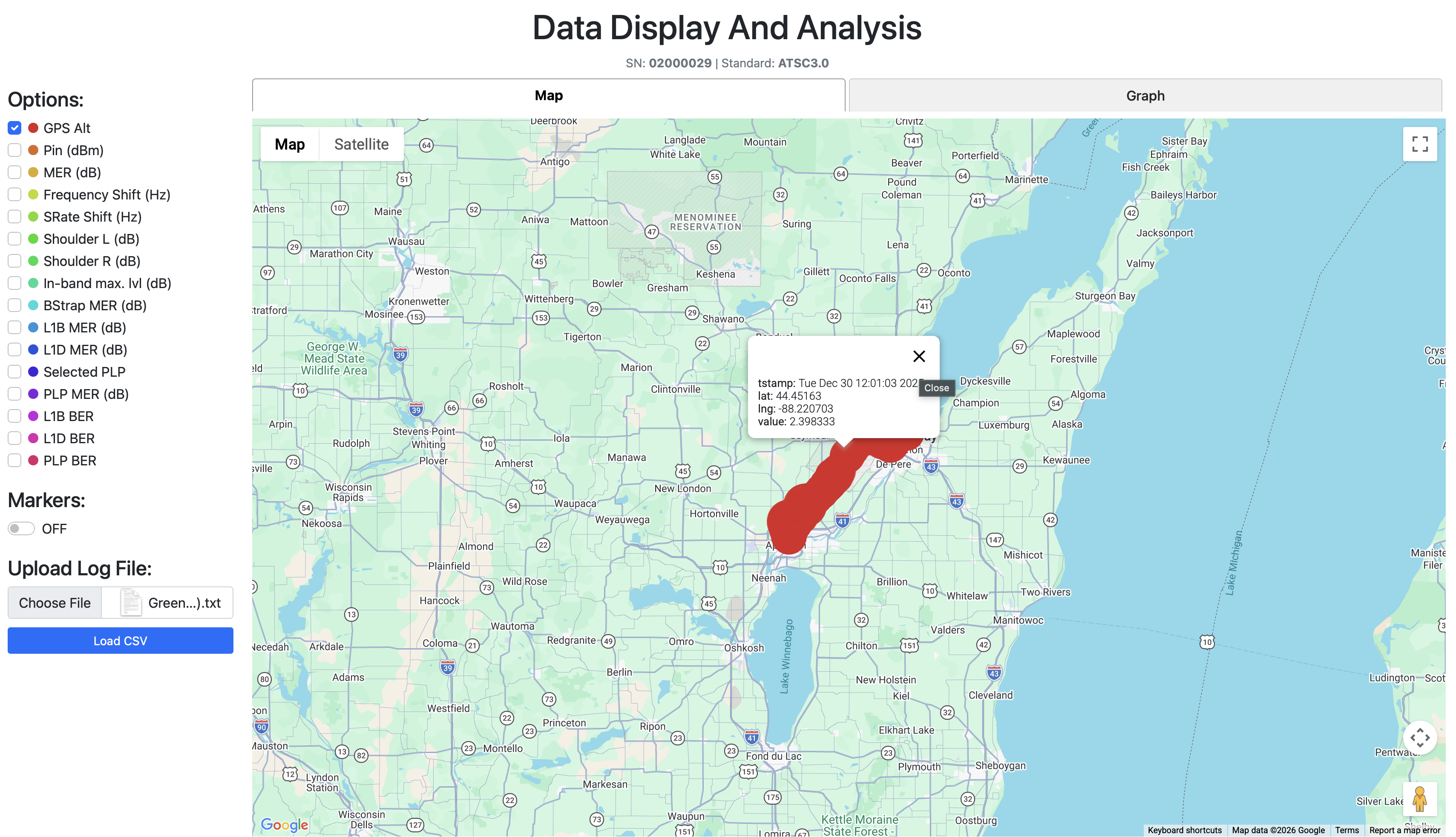
GMAP Version 3 worked.
Let me say that more clearly - it actually worked. Drive test data on a map, FSPL predictions overlaid, Hata-Okumura terrain correction applied, NLCD land cover tiles processed, threshold visualization, a polished UI. Company branding. The whole thing.
I was proud of it.
But there was this quiet feeling that kept showing up whenever I looked at the coverage polygons - these perfectly smooth, mathematically clean circles spreading outward from the transmitter like ripples in a pond. Neat. Predictable. A little too perfect.
The real world doesn't look like that.
Hata-Okumura is an empirical model from the 1960s. It classifies terrain into broad categories - urban, suburban, rural - and applies correction factors accordingly. A mountain range between the transmitter and receiver? A valley? A river?
Hata doesn't care. It sees "suburban" and applies the formula.
For ATSC 3.0 broadcast coverage - where you're pushing megawatts of ERP over 100+ km from 300m towers - that's not good enough.
This is the story of how I fixed that.
The Moment That Started Everything
The CEO was preparing a presenting to present to clients. He was going through the slides, re-reading through the coverage capabilities, when he landed on a specific picture - a full map of the USA, blanketed in broadcast station coverage overlays.
Clean circles. Smooth edges. Very Hata.
Right under that image, a small label described which propagation model this map had used. He called me over.
"Look into this model. Maybe it will help getting that perfect prediction you're looking for."
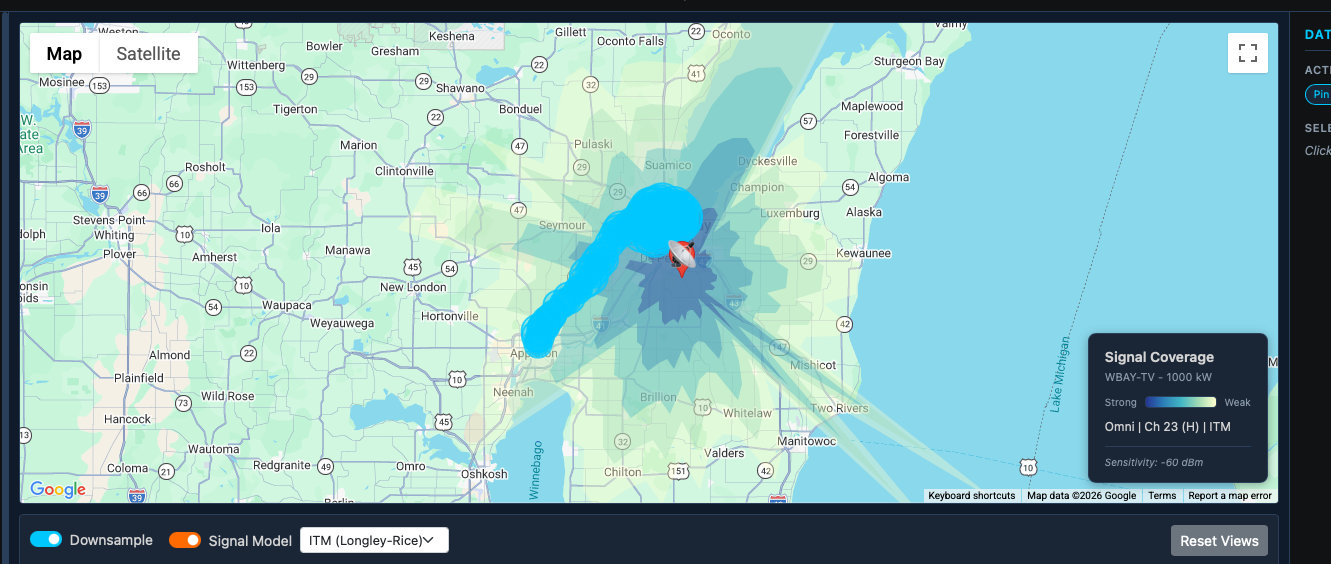
The model was called ITM. The Irregular Terrain Model.
I opened it on my laptop. And I stared.
The coverage polygons were nothing like mine. They weren't circles. They weren't smooth. They looked like someone had torn paper - ragged, asymmetric, full of gaps and holes where terrain blocked signal. Every single one was different.
That's it, I thought. That's what real coverage actually looks like.
Moving Everything to the Backend
Before I could touch ITM, I had to solve a different problem.
The frontend was doing everything - Hata calculations, NLCD lookups, terrain segment analysis, all in JavaScript. This worked for simple models. But ITM is a different beast. It needs:
- SRTM elevation data (~2.4 GB of terrain tiles, memory-mapped)
- NumPy array operations for profile analysis
- The
itmlogicPython library - a port of the original Fortran code - Heavy computation per radial (up to 600 elevation samples per path)
None of that runs in a browser.
So I set up a Flask API backend. The frontend became a thin client - send a station ID and model selection, receive pre-computed polygons and signal predictions, render them. All heavyweight work happens server-side.
I also restructured the backend into proper singleton services: TerrainService, SrtmService, ItmService, PropagationService, CoverageService. The singleton pattern matters here because ItmService opens the 2.4 GB SRTM binary on initialization - you want that to happen once at startup, not once per request:
class ItmService:
    _instance = None

    def __new__(cls):
        if cls._instance is None:
            cls._instance = super().__new__(cls)
            cls._instance._initialized = False
        return cls._instance

    def __init__(self):
        if self._initialized:
            return
        self._srtm = SrtmService()   # opens 2.4 GB mmap - once, ever
        self._check_itm_library()
        self._initialized = True
The architecture was ready. The model wasn't.
Actually Understanding ITM
The Irregular Terrain Model - also called Longley-Rice - is the propagation model the FCC uses for broadcast TV coverage prediction. Physics-based. Developed at the Institute for Telecommunication Sciences in the 1960s-70s. It actually traces radio waves over real terrain profiles.
Here's where I hit my first wall.
The itmlogic package's __init__.py exports nothing useful. You can't just import itmlogic and call a function. You have to import three specific internal modules:
from itmlogic.misc.qerfi import qerfi                        # inverse normal CDF
from itmlogic.preparatory_subroutines.qlrpfl import qlrpfl  # terrain profile analysis
from itmlogic.statistics.avar import avar                    # statistical variability
No high-level "calculate path loss" function exists. You build a prop dictionary yourself, compute intermediate electromagnetic quantities by hand, feed in the terrain profile in a specific format, and chain all three functions together. Here's what the electromagnetic setup looks like:
# Wave number: converts frequency to spatial wavelength
prop['wn'] = frequency_mhz / 47.7

# Effective Earth curvature (accounts for atmospheric refraction)
# ens = 301 N-units (BPS/TVStudy standard - not 314, which I had wrong)
prop['gme'] = prop['gma'] * (1 - 0.04665 * math.exp(prop['ens'] / 179.3))

# Complex ground impedance
# Average ground: eps=15.0, sgm=0.005 S/m
# Water paths:    eps=80.0, sgm=4.0 S/m  (dramatically different behavior)
zq = complex(prop['eps'], 376.62 * prop['sgm'] / prop['wn'])
prop['zgnd'] = np.sqrt(zq - 1)
I had no idea going in. Not even a little bit.
But here's the thing about a model this complex - you can't just plug numbers in and hope. The moment you misunderstand one parameter, every prediction shifts. So before writing a single line of integration code, I went through the math layer by layer. Here's what I found.
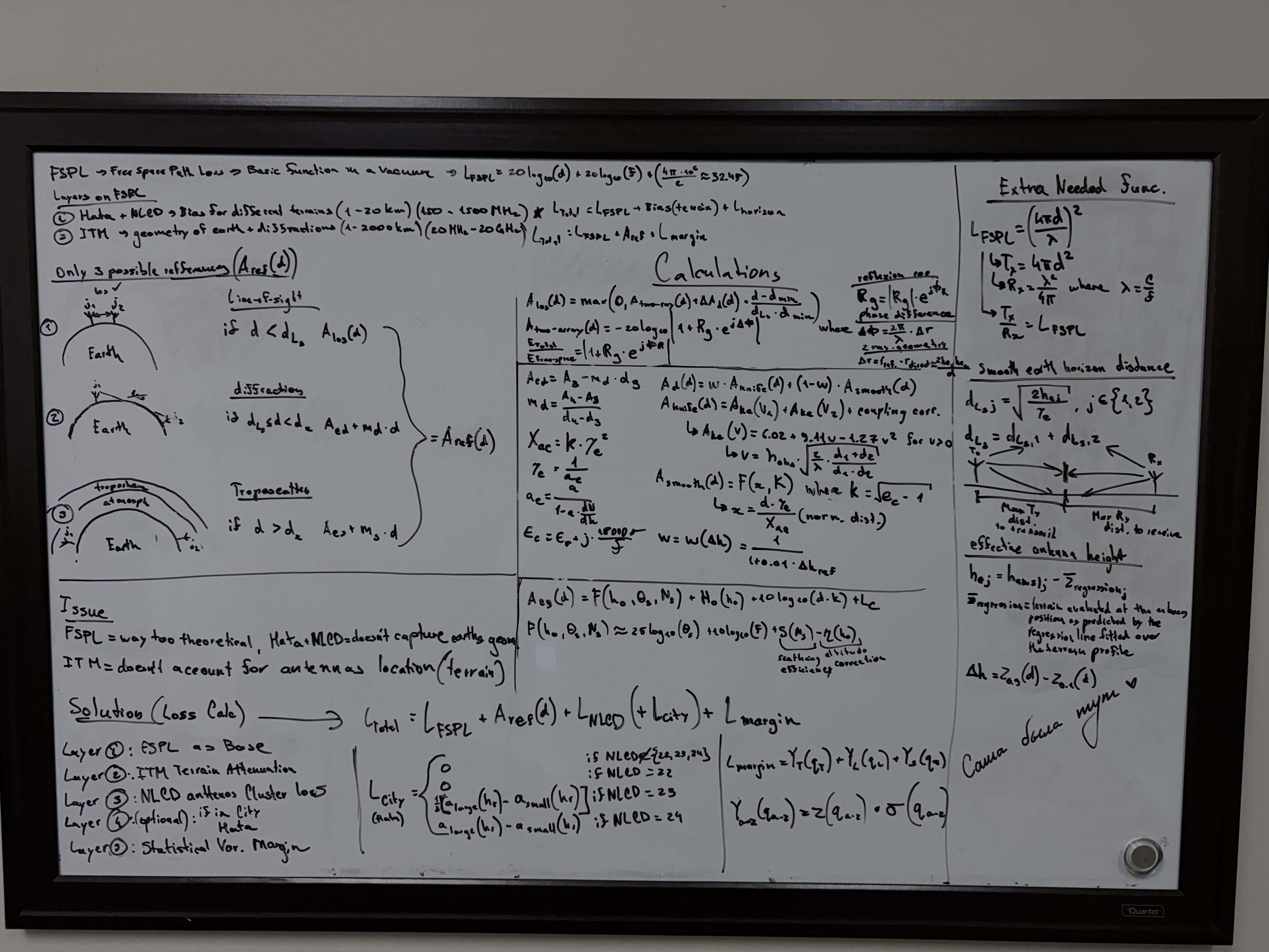
The Math - Walking Through ITM From Scratch
Think of it in layers.
FSPL is signal loss in a perfect vacuum - nothing between transmitter and receiver. Just distance and frequency. Clean and simple. If the universe were empty air, this would be enough.
ITM is everything on top of that. The total output is called A_ref - reference attenuation above free space, caused by terrain interaction. Here's how it gets computed.
The Earth Isn't Flat - Effective Earth Radius
Radio waves don't travel in straight lines. The atmosphere bends them slightly downward, which actually helps - signals can reach slightly beyond the geometric horizon.
ITM models this by replacing the real Earth radius with an effective radius:
The standard value of N-units gives the classic 4/3 Earth - a "fatter" planet that captures real propagation paths without modeling the atmosphere explicitly. The effective Earth curvature becomes .
This is where I found a bug in the existing tool. I was using instead of 301. It shifts the curvature term, which shifts every horizon distance calculation, which shifts every single prediction.
Smooth Earth Horizon Distance
Before looking at any real terrain, ITM establishes the maximum range over a perfectly smooth Earth:
Each antenna sees out to its own geometric horizon. Add them together - that's , the boundary between line-of-sight and diffraction regime. For a 300m tower transmitting to a 1.5m portable receiver:
Beyond 76 km, there's no direct ray. The signal has to bend over terrain.
Effective Antenna Heights - Not Just "How Tall Is the Tower"
ITM doesn't use physical antenna height. It fits a least-squares regression line through all elevation samples along the path and measures the antenna's height above that regression line - not above the ground directly beneath it.
If a transmitter sits on a hillside, its physical height above ground might be 50m. But if that hillside rises steeply, the effective height above the dominant terrain slope might be 200m - and that's what actually determines propagation.
Terrain Irregularity (Δh) - How Rough Is the Ground?
ITM captures terrain roughness in a single number:
The 90th percentile elevation deviation minus the 10th. Discard the extreme top and bottom 10% of terrain heights, measure the spread of what's left. Flat terrain → Δh near zero. Mountainous terrain → large Δh. This single parameter controls the blend between two diffraction models.
The 3 Regimes - Distance Determines Everything
This is the core of A_ref. Depending on how far the receiver sits relative to , ITM switches between three completely different physical mechanisms:
In the three-stage ITM calculation, these regimes are evaluated like this:
# Stage 1: Terrain analysis - scans profile, finds horizon points,
# determines propagation mode (LOS / diffraction / troposcatter)
prop = qlrpfl(prop)

# Stage 2: Free-space baseline
db = 8.685890  # = 20 / ln(10), converts nepers to dB
fs = db * np.log(2 * prop['wn'] * prop['dist'])

# Stage 3: Terrain and statistical effects (the A_ref term)
zr = qerfi([0.5])   # z-score at 50th percentile = 0 (median prediction)
avar1, prop = avar(zr[0], 0, zr[0], prop)

total_loss = float(fs + avar1)
In line-of-sight, the signal arrives via two simultaneous paths - a direct ray and a ground reflection. These interfere. In phase: constructive addition. Out of phase: cancellation. This is why signal strength doesn't smoothly decay with distance - it oscillates with peaks and nulls.
In the diffraction regime, there's no direct ray. ITM computes two types of diffraction and blends them by terrain roughness:
Smooth Earth diffraction handles gently rolling terrain. Knife-edge diffraction (using the Fresnel-Kirchhoff parameter ) handles sharp ridges. The blend: rough terrain → → knife-edge dominates. Smooth terrain → → smooth Earth dominates.
Troposcatter matters for paths well beyond the horizon where signal scatters off atmospheric turbulence. For most ATSC 3.0 scenarios it's rarely dominant, but I implement it for completeness.
I run ITM in broadcast mode:
prop['mdvarx'] = 13 # broadcast (3) + wide loss flag (+10)
Mode 3 assumes a fixed transmitter and varying receiver locations - exactly the broadcast TV scenario. The +10 wide loss flag uses a more conservative statistical distribution, matching FCC TVStudy 2.3.0's behavior.
Where NLCD and Hata Come In
ITM is purely physics plus terrain geometry. It reads elevation profiles. It cannot see what's sitting on top of the terrain - buildings, trees, urban density. SRTM3 (the elevation dataset) is bare Earth. A downtown skyscraper is invisible to it.
So after ITM gives me A_ref, I add an obstruction penalty for above-ground loss. For urban areas, I use the difference between Hata's environment-specific loss and Hata's rural baseline:
def calculate_obstruction_penalty(nlcd_code, distance_km, freq, tx_h, rx_h):
    if category == 'open':
        return 0.0  # water, barren, grassland - nothing above ground blocks signal

    if category.startswith('dev_'):
        rural_loss = calculate_rural_loss(d, freq, tx_h, rx_h)
        env_loss   = calculate_urban_loss(d, freq, tx_h, rx_h, city_type)
        return max(0.0, env_loss - rural_loss)  # DIFFERENCE = building loss only
Why the difference? The full Hata urban formula captures both terrain effects AND building effects. The rural formula captures terrain only. Subtracting them isolates the building contribution - and it varies naturally with frequency, distance, and antenna heights. Not a fixed lookup table.
For vegetation, frequency-dependent attenuation scaled by canopy density:
FOREST_ATTENUATION = {
    'vhf_low':  3,  # 54-88 MHz  - long wavelength, punches through foliage
    'vhf_high': 5,  # 174-216 MHz
    'uhf':      8   # 470-700 MHz - short wavelength, absorbed by leaves
}
# Canopy density scaling: evergreen 100%, mixed 85%, deciduous 70%, shrub 30%
Open terrain - water, grassland, barren land - gets zero penalty. A 1.5m receiver in a field has nothing above ground to block it.
The full penalty is then scaled by 0.2 before adding to ITM loss:
ITM_CLUTTER_BIAS = 0.2 # 20% of raw penalty on top of ITM
Why 0.2? The full Hata obstruction penalty accounts for aggregate propagation effects that ITM already partially models through SRTM terrain profiles. The 0.2 scaling was calibrated against drive test measurements - it minimizes the mean prediction error for my dataset.
Statistical Margins - Because Reality Varies
A prediction of "-50 dBm" is a median. For 90% reliable broadcast coverage, I add a margin:
Where is the inverse normal CDF at 90% confidence. I implement this without scipy using the Abramowitz & Stegun rational approximation (accurate to ~4.5×10⁻⁴):
t = math.sqrt(-2 * math.log(1 - p))
c0, c1, c2 = 2.515517, 0.802853, 0.010328
d1, d2, d3 = 1.432788, 0.189269, 0.001308
z = t - (c0 + c1*t + c2*t*t) / (1 + d1*t + d2*t*t + d3*t*t*t)

# z(0.5) = 0.0    (median - no margin)
# z(0.9) = 1.282  (standard broadcast reliability)
# z(0.95) = 1.645 (conservative)
dB (time variability - atmospheric conditions day to day), dB (situation variability - different installations). Location variability is dropped for the ITM model since the clutter layer already captures most of it.
The complete signal budget for one receiver point:
P_rx = ERP_dBm + antenna_pattern_dB - (L_itm + L_clutter + L_margin)

Example: 1,000 kW station, ch.29 (563 MHz), 300m tower, 50km suburban (NLCD 22)
  ERP_dBm     = 10 * log10(1000 * 1e6)  = 90.0 dBm
  L_itm       ≈ 140 dB (terrain-dependent)
  L_clutter   ≈ 1.2 dB (suburban Hata differential * 0.2)
  L_margin    = 1.282 * 1.5 + 1.282 * 1.5 = 3.85 dB
  P_rx        = 90.0 - 145.05 = -55.05 dBm
  Threshold   = -60 dBm → coverage confirmed
Once I had all of this in my head - actually understood what each piece was doing - plugging it into itmlogic made sense. You're not calling a function. You're building the physics layer by layer. That's the only thing that makes the bugs debuggable when they appear.
SRTM - 2.4 GB of Real Terrain
ITM needs actual elevation data. I used NASA's SRTM3 - ~90m horizontal resolution, globally.
The challenge: SRTM comes as ~1,800 individual 1-degree tiles for CONUS coverage, each 1201×1201 pixels at 2 bytes per pixel (~2.88 MB each). Managing thousands of loose files is a nightmare for both storage and access latency.
So I packed everything into a single binary file with a JSON index:
srtm_elevation.bin (2.4 GB):
┌─────────────────┬─────────────────┬─────────────────
│  Tile N24W067   │  Tile N24W068   │  Tile N24W069  ...
│  2,884,802 B    │  2,884,802 B    │  2,884,802 B
└─────────────────┴─────────────────┴─────────────────

srtm_elevation.json:
{ "tiles": { "N40W074": 0, "N40W075": 2884802, ... } }
To read an elevation at a given lat/lon, it's a four-step lookup:
# 1. Which tile? Floor the coordinates → e.g., lat=40.7, lon=-74.1 → "N40W074"
tile_name = f"N{int(lat):02d}W{abs(int(lon)):03d}"

# 2. Sub-tile pixel position (row 0 = NORTH edge - tiles are named by SW corner)
row = int((1.0 - lat_frac) * (pixels - 1))  # inverted: higher lat → lower row
col = int(lon_frac * (pixels - 1))

# 3. Byte offset into the binary file
byte_offset = tile_start + (row * 1201 + col) * 2

# 4. Read 2 bytes - big-endian signed int16
elevation = struct.unpack('>h', data[byte_offset:byte_offset + 2])[0]
# -32768 = SRTM void (ocean or missing tile)
Access is memory-mapped for speed. On production (cPanel/Passenger), mmap sometimes fails silently on large files - so I detect the failure once and fall back permanently to file-seek reads:
try:
    self._packed_mmap = mmap.mmap(file.fileno(), 0, access=mmap.ACCESS_READ)
    _ = self._packed_mmap[test_offset:test_offset + 2]  # verify it actually works
except Exception:
    self._use_file_seek = True  # slower, but universally compatible
For terrain profiles, I sample along true great-circle paths using the haversine forward formula - not linear lat/lon interpolation. This matters because linear interpolation shifts all intermediate points depending on the path's total length. Two calls to the same bearing at 17 km would return different coordinates depending on whether I was computing a 22 km or 150 km profile. Great-circle sampling is path-length-independent.
Terrain profiles use adaptive resolution to match TVStudy's approach:
# 2 points per km, bounded [20, 600]
num_points = max(20, min(600, int(distance_km * 2)))

#   5 km path → 20 points  (250m spacing - minimum)
#  50 km path → 100 points (500m spacing)
# 300 km path → 600 points (500m spacing - at the cap)
SRTM3 has ~90m resolution. At 500m spacing, I'm sampling every ~5 pixels - enough to capture significant terrain features without wasting computation on subpixel precision I don't have.
The Spiky Graph Problem
This is the debugging session I remember most.
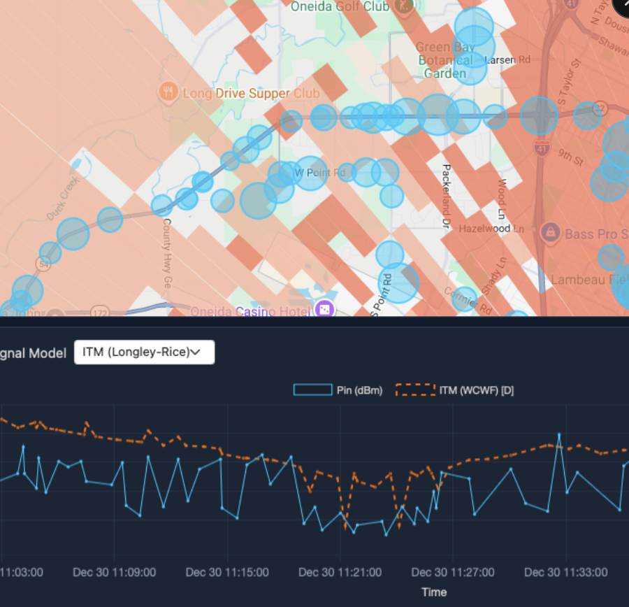
After all five layers were active - ITM, SRTM terrain profiles, NLCD clutter, Hata urban correction, statistical margins - I pulled up the signal prediction graph against a drive test dataset.
It looked like an EKG. Wild 15–20 dB spikes at nearly every point. I had been working on this for days. I knew what every layer was doing. And I genuinely could not explain what I was looking at.
"How is this possibly correct?"
It wasn't. Three things were compounding each other.
Problem 1: Double urban penalty. NLCD clutter loss AND the Hata urban correction were both being applied to the same areas. Dense urban (NLCD code 24) was taking 18 dB of clutter loss plus a separate Hata large-city correction on top. Cities were being penalized twice for the same buildings.
Problem 2: Non-standard clutter values. The NLCD_CLUTTER_TABLE used custom dB values that weren't from any published standard, causing arbitrary 0–18 dB jumps at every 500m NLCD cell boundary.
Problem 3: Resolution mismatch. At 0.005-degree NLCD resolution (~555m per pixel), two adjacent drive test points straddling a pixel boundary would see completely different clutter values - sharp 8–15 dB discontinuities, hundreds of times per profile.
The fix: throw out the separate clutter and urban layers entirely. Replace with a single calculate_obstruction_penalty() function that uses the Hata differential for urban, frequency-scaled attenuation for vegetation, and zero for open terrain. Then scale everything by ITM_CLUTTER_BIAS = 0.2.
I also fixed three drifted parameters I caught while I was in there:
| Parameter | Was | Fixed To | Why |
|---|---|---|---|
| Surface refractivity () | 314 N-units | 301 N-units | TVStudy/BPS standard |
| RX antenna height | 10 m AGL | 1.5 m AGL | Realistic portable reception |
| in margin formula | Included | Dropped | Clutter layer now covers location variability |
The graph went smooth. That was a very good moment.
Matching the FCC
After the graph stabilized, I ran a gap analysis against FCC TVStudy 2.3.0 - the government's official broadcast coverage tool. Several things were still off.
ITM broadcast mode. I was using mdvarx=11 (Individual mode). TVStudy uses mdvarx=13 (Broadcast mode + wide loss flag). Individual mode assumes both transmitter and receiver locations vary. Broadcast mode assumes only the receiver varies - the right assumption for a fixed tower broadcasting to a roaming audience.
Water path detection. Water has dramatically different electromagnetic properties - permittivity 80 vs 15, conductivity 4.0 vs 0.005 S/m. Signals genuinely travel farther over water. I added NLCD sampling along each path:
def _detect_water_path(self, tx_lat, tx_lon, bearing, distance_km, num_samples=5):
    sample_max = 30.0  # km cap - check near-field regardless of total path length
    water_count = 0
    for i in range(1, num_samples + 1):
        d = sample_max * i / (num_samples + 1)
        pt = destination_point(tx_lat, tx_lon, bearing, d)
        if terrain.query_nlcd(pt['lat'], pt['lon']) == 11:  # NLCD "Open Water"
            water_count += 1
    if water_count / num_samples >= 0.5:
        prop['eps'] = 80.0   # override: average ground → water
        prop['sgm'] = 4.0
The 30 km cap is critical. Without it, a 150 km radial over Lake Erie would sample points far offshore, while a 22 km radial would sample near the transmitter. The same station would get different water detection results depending on path length - I traced a 33 dB discrepancy between the coverage polygon and the batch-signal graph at the same bearing. All caused by this single inconsistency.
Antenna pattern interpolation. Directional patterns were being applied to coverage polygons but not to batch signal predictions. The graph was omnidirectional while the polygon was directional. I also found 20–30 dB erratic jumps at bearing bucket boundaries - two adjacent drive test points at 45.9° and 46.1° were snapping to completely different terrain profiles. Fix: linear interpolation between adjacent 1-degree profiles:
b_lo  = int(bearing) % 360
b_hi  = (b_lo + 1) % 360
frac  = bearing - int(bearing)  # 0.0 to 1.0

# bearing 45.7°: 30% profile-45, 70% profile-46
itm_loss = loss_lo + frac * (loss_hi - loss_lo)

# Before: 20-30 dB jumps at bearing boundaries
# After:  smooth interpolation between adjacent profiles
The Coverage Polygon Journey
This was a visual journey through three completely different ideas - and the most satisfying problem I solved on this project.
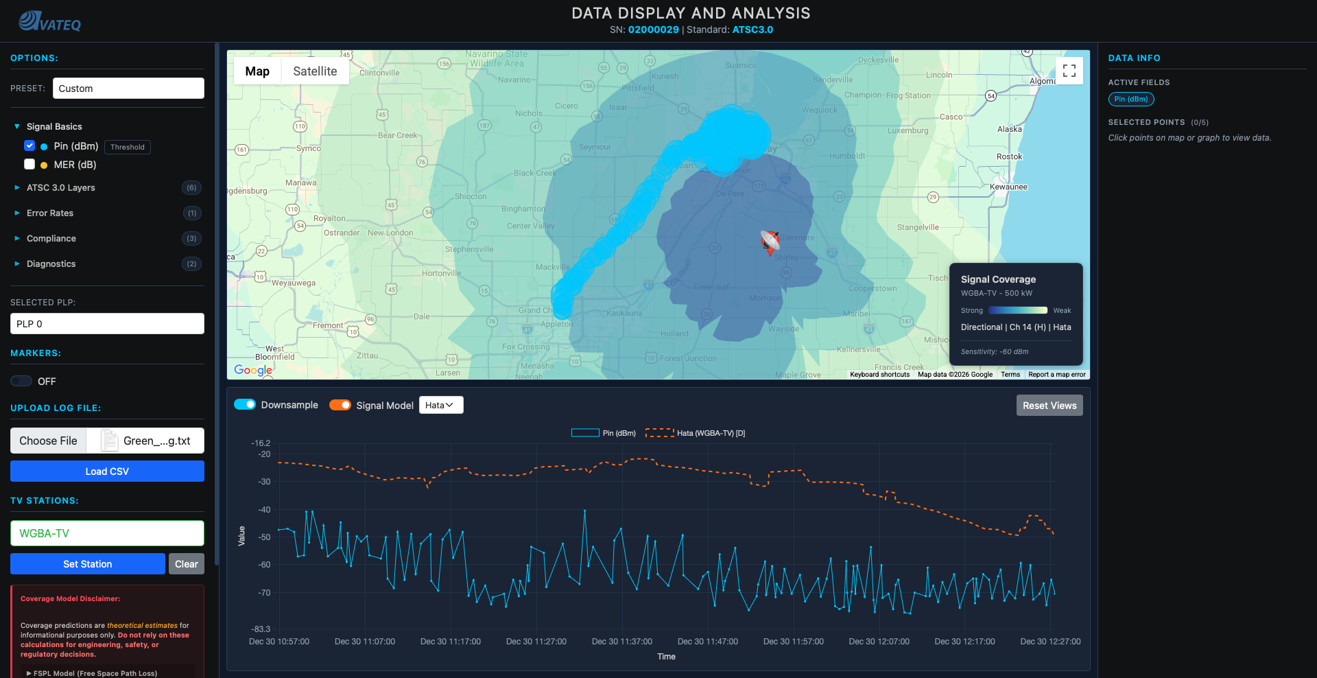
Attempt 1: Contour rings. Walk each of 360 radials until signal drops below threshold. Connect those points into a smooth ring.
Pretty. Clean. Wrong. The rings averaged everything out. If a mountain blocked signal at bearing 270° but not 271°, the ring smoothed over it. ITM's entire purpose is terrain awareness - and my visualization was hiding it.
Attempt 2: Clustered wedge polygons. Per-point coloring. Same-color adjacent points merge into wedges. Signal below threshold = no polygon = natural shadow zone.
This showed the terrain. Gaps appeared where mountains blocked signal. It looked right.
Problem: ~1,500 tiny wedge polygons per station. Google Maps slowed to a crawl. Zooming stuttered. Edges looked jagged.
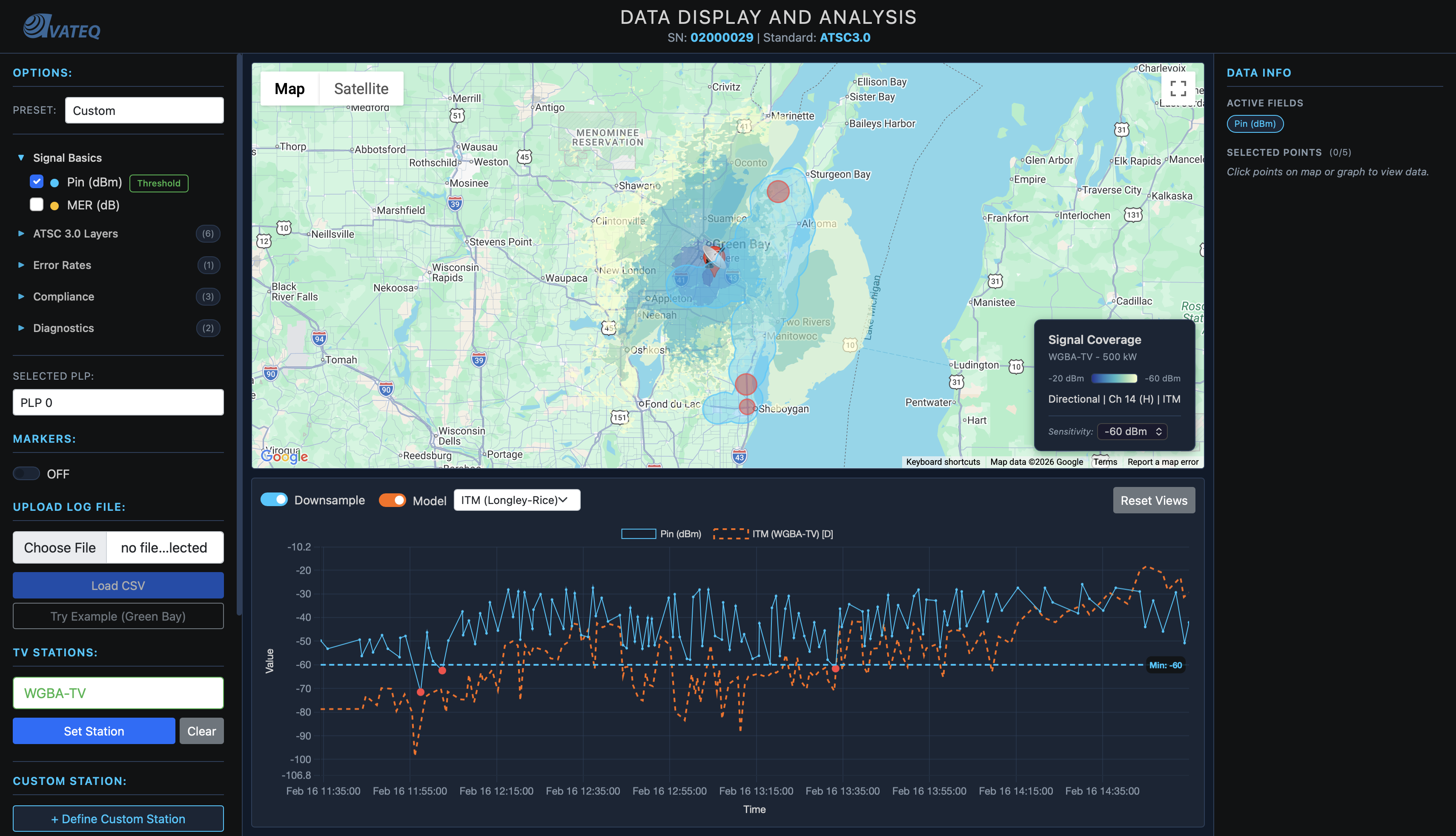
Attempt 3: Contourf. The solution that combined both:
# Step 1: 360 radial profiles → 500x500 Cartesian signal grid
grid_res = 500
xi = np.linspace(-max_d, max_d, grid_res)
XI, YI = np.meshgrid(xi, xi)

# For each grid point, find adjacent bearing profiles and blend
ZI[mask] = prx_lo * (1 - frac) + prx_hi * frac  # same math as batch-signal

# Step 2: Extract smooth contour polygons (holes = shadow zones)
fig, ax = plt.subplots(figsize=(1, 1))
cs = ax.contourf(XI, YI, ZI, levels=[-60, -50, -40, -30, -20], extend='max')
plt.close(fig)   # ← never render - I just want the geometry

# Step 3: Convert km offsets → lat/lon
# paths[0] = outer boundary, paths[1:] = holes (terrain shadow zones)
# → google.maps.Polygon with even-odd fill rule handles holes automatically
The key insight: use matplotlib's contourf as a computational geometry tool, not for plotting. Create the figure in memory. Extract the contour paths. Close the figure. Never render it. matplotlib doesn't know it's being used this way - it just does the geometry and hands back polygon coordinates.
Result: ~1,500 tiny wedge polygons → ~5 smooth multi-path polygons. Shadow zones appear as holes. Rendering is instant. 100x fewer DOM elements, smooth edges, terrain awareness preserved.
The Performance Architecture
When a user selects a station, the frontend fires four API requests simultaneously - no sequential waiting:
const [itmCoverage, fsplCoverage, itmSignal, fsplSignal] = await Promise.all([
    coverageApiPolygonPost(station, 'itm'),   // ~3-5 seconds (heavy terrain computation)
    coverageApiPolygonPost(station, 'fspl'),  // ~50ms  (simple circle)
    coverageApiBatchSignal(station, 'itm'),   // ~2-3 seconds
    coverageApiBatchSignal(station, 'fspl')   // ~100ms
]);
// FSPL renders immediately. ITM swaps in when ready. Model toggle = instant cache swap.
The batch-signal endpoint uses the radial optimization - one terrain profile per bearing, shared across all distance steps:
# Extract FULL profile along each bearing once (the expensive part: disk I/O)
full_profile, step_km = srtm.get_elevation_profile_along_bearing(
    tx_lat, tx_lon, bearing, max_distance_km, num_profile_points
)

# Then reuse subsets for each distance step (just arithmetic, no more I/O)
for i in range(min_points, num_profile_points + 1):
    profile_subset = full_profile[:i + 1]  # truncate, don't re-extract
    itm_loss = run_itm(profile_subset, ...)
Without it: 360 bearings × 300 distance steps = 108,000 SRTM binary reads. With it: 360 reads + 108,000 ITM calculations on already-loaded data.
Terrain extraction is the expensive operation (disk I/O from a 2.4 GB binary). That's a ~300× I/O reduction.
Results are cached at four levels:
Level 1: ITM point cache        - 5,000 entries, keyed by quantized TX/RX coords + params
Level 2: SRTM tile cache        - 8 tiles in memory (~24 MB), LRU eviction
Level 3: Coverage polygon cache - 50 results, full polygon JSON
Level 4: Frontend model cache   - both ITM + FSPL in JS, model toggle = DOM swap, no API call
The Canvas Rendering Rewrite
Before this rewrite, the map was painfully laggy. Every pan was slow. Every zoom stuttered. With 10,000+ drive test points loaded, interacting with it felt like dragging wet cardboard.
After: 60 fps.
The change was entirely in how I render data circles.
The old way: every data point was a google.maps.Marker object. Each marker creates a DOM element, an SVG symbol, a selected symbol, an InfoWindow instance, and multiple event listeners. With 10,000 points:
10,000 DOM elements       (one per data point)
20,000 SVG symbol objects (normal + selected state)
10,000 InfoWindow instances
20,000+ event listeners
Google Maps had to reposition all of them on every pan and zoom event. Toggling a data field (destroying all markers, recreating them) took visible seconds.
The new way: replace every marker with a plain JavaScript descriptor - no DOM, no API objects, no event listeners:
const desc = {
    lat: item.lat, lng: item.lng,
    latLng: new google.maps.LatLng(item.lat, item.lng),
    worldX: 0, worldY: 0,       // pre-computed once on load, reused every frame
    radius: pixelRadius,         // visual size in pixels
    color: markerColor,          // '#ff4444' for threshold violations
    baseFillOpacity: 0.55,       // 0.75 for violations (more visible)
    dataIndex: dataIndex,        // index into appData[] for click info window
    isSelected: false
};
A single google.maps.OverlayView subclass creates one HTML5 <canvas> covering the entire viewport. Every frame, it redraws all circles in one pass.
The critical performance insight: Google Maps uses a "world coordinate" system where the entire planet fits in a 256×256 grid at zoom 0. These coordinates are zoom-invariant - they never change regardless of pan or zoom.
// Compute ONCE when data loads
const wp = mapProj.fromLatLngToPoint(c.latLng);
c.worldX = wp.x;   // e.g., 69.234 (never changes)
c.worldY = wp.y;   // e.g., 95.118

// Per frame: 4 API calls for viewport corners → derive linear transform
const scaleX = (ne.x - sw.x) / (neW.x - swW.x);
const divX   = sw.x + (c.worldX - swW.x) * scaleX;  // 2 multiplies + 2 adds per circle
Before: 10,000 calls to fromLatLngToDivPixel() per frame.
After: 4 API calls + 10,000 arithmetic operations. Arithmetic is ~1,000× faster than API calls.
Drawing 10,000 semi-transparent circles onto a single canvas creates alpha stacking - overlapping circles compound and get darker than intended, and internal borders look ugly where circles meet. The fix uses two offscreen canvases and composite operations:
// Canvas A: all same-color circles as opaque fills
a.fillStyle = color;
for (const c of items) { a.arc(c.x, c.y, c.r, 0, Math.PI * 2); a.fill(); }

// Canvas B: borders, then erase interior halves
b.strokeStyle = color; b.lineWidth = 3.5;
for (const c of items) { b.arc(c.x, c.y, c.r, 0, Math.PI * 2); b.stroke(); }

b.globalCompositeOperation = 'destination-out';  // "punch holes wherever I draw"
for (const c of items) { b.arc(c.x, c.y, c.r, 0, Math.PI * 2); b.fill(); }  // erase interiors

// Composite to main canvas
ctx.globalAlpha = fillOpacity;   ctx.drawImage(offA, ...);  // fills at fill opacity
ctx.globalAlpha = strokeOpacity; ctx.drawImage(offB, ...);  // outer borders only
The destination-out trick erases any border pixels that fall inside any circle. Where circles overlap, the internal borders vanish and the regions look like one cohesive filled area.
For click detection with no Marker event listeners, I use a spatial hash grid: after each render, every visible circle registers in a 50×50 pixel cell. Click → look up the cell → check the 3×3 neighborhood → find the closest circle:
// Squared distance comparison - no sqrt() needed
const dist = dx * dx + dy * dy;
if (dist <= c.radius * c.radius && dist < bestDist) { best = c; }
Average: ~27 distance comparisons. O(1) amortized vs O(n) for scanning all 10,000 circles. The 3×3 neighborhood is necessary because a circle centered near a cell boundary extends into adjacent cells - checking only the clicked cell would miss it.
Circles outside the visible viewport are skipped entirely before drawing and before grid registration:
if (x + c.radius < 0 || x - c.radius > w ||
    y + c.radius < 0 || y - c.radius > h) continue;  // viewport culling
At typical zoom levels, 50–80% of circles are off-screen. Culling them saves both draw calls and spatial grid memory.
BEFORE → AFTER
10,000 DOM elements      → 1 canvas element
10,000 InfoWindows       → 1 shared InfoWindow
20,000+ event listeners  → 3 event listeners
Laggy pan/zoom           → 60 fps
That was a good day.
The CORS Bug That Took Too Long
I'll keep this one short because the fix was embarrassingly simple.
After adding API security - key-based authentication (X-API-Key header), rate limiting (60 req/min default, 10 req/min for heavy coverage endpoints), and origin validation - the site broke. 403 errors everywhere. The X-API-Key header wasn't being sent even though the client code was updated.
It worked perfectly in incognito. Nowhere else.
Root cause: CORS preflight caching. The old config had max_age: 86400 (24 hours). The browser had cached a preflight response that didn't include X-API-Key in Access-Control-Allow-Headers. On every subsequent request, it checked the cache, saw the header wasn't permitted, stripped it silently, and the server rejected the request with 403.
Fix: reduce max_age from 86400 to 3600. Wait for the cache to expire.
That's it. The incognito clue was there the whole time - fresh session, no cached preflight, everything worked.
I stared at this for longer than I'm willing to admit.
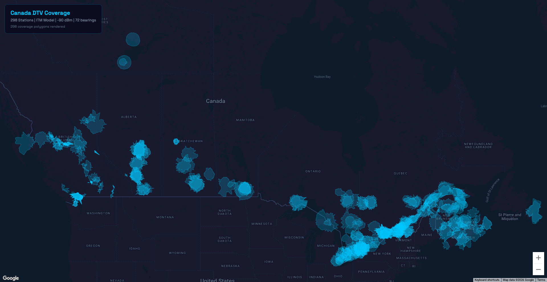
Canada Expansion
Users wanted to see Canadian stations. So I added them.
388 stations from ISED's broadcasting database - 253 full-power, 135 low-power - with ERP, HAAT, coordinates, and 276 directional antenna patterns. Total station count: 2,165 US → 2,553.
For terrain, I extended the SRTM download to N42–N59, W52–W141. Tiles: ~1,800 → ~2,682. For land cover, I sourced the 2020 Land Cover of Canada dataset, remapped Canadian codes to NLCD equivalents, and created a separate terrain_canada.bin. The TerrainService queries US data first, falls back to Canadian if the result is nodata (code 250):
def query_with_fallback(self, lat, lon):
    result = self.query_us(lat, lon)
    if result == 250:  # SRTM void - not necessarily outside US bounds
        result = self.query_canada(lat, lon)
    return result
The bug that appeared immediately: Toronto (lat 43.6°N) falls within the US terrain binary's geographic bounds but returns nodata 250 - the tile exists in the index but has no actual coverage data. The original code wasn't treating 250 as a fallback trigger. It returned 250 as a valid land cover code, corrupted the NLCD lookup, and broke every coverage polygon for stations along Lake Ontario.
One condition check. Fixed.
The Full Picture
What I Built
From V3 - Hata overlays, smooth prediction circles, rough signal estimates - to a production-deployed ITM coverage engine with real terrain diffraction, shadow zone visualization, Canadian station support, custom station analysis, API security, and a canvas renderer handling 15K+ drive test points at 60 fps.
The ragged, torn-paper polygons from that presentation turned out to be more than a visual trick. They were the honest shape of what radio actually does over real terrain. Every dip and hole in the coverage map is a mountain, a ridge, a valley doing what physics says it should.
That's the thing about getting the math right. The map stops being a diagram and starts being a picture of something real.
Tech stack: Python/Flask API backend, itmlogic (Longley-Rice ITM), SRTM3 elevation data (2.4 GB memory-mapped binary), NLCD + Canadian land cover databases, Google Maps API with custom OverlayView canvas renderer, matplotlib (contourf for polygon geometry), Vanilla JavaScript frontend, 4-level caching architecture.
Limitations & Caveats
Being transparent about what this tool still does NOT do:
- Predicted signal sometimes drops below measured data. At certain points, the ITM prediction is lower than what drive tests actually recorded. I still don't fully understand why. Maybe the station is just outperforming free-space path loss - someone tell the physics department they need to update the laws of electromagnetic propagation.
- SRTM resolution caps terrain detail. SRTM3 gives ~90m horizontal resolution. A narrow canyon, a single building, or a tree line between two sample points is invisible. At 500m profile spacing, I'm capturing terrain features at ~5-pixel resolution - enough for ridges and valleys, not enough for street-level accuracy.
- No atmospheric modeling. Temperature inversions, ducting, rain fade, and seasonal refractivity changes aren't accounted for. The surface refractivity is fixed at 301 N-units year-round. In reality, it varies by season, weather, and geography.
- No interference analysis. Co-channel and adjacent-channel interference from neighboring stations isn't modeled. A point might show strong signal but be unusable because three other stations are competing on the same frequency.
- The 0.2 clutter bias is empirically tuned.
ITM_CLUTTER_BIAS = 0.2was calibrated against one set of drive test data. It minimizes mean error for that dataset. Different regions, different station configurations, different receiver environments - it may not generalize. - Contourf polygon resolution is fixed. The 500×500 Cartesian grid determines polygon smoothness. Small shadow zones narrower than one grid cell get averaged out. Increasing resolution would improve accuracy but increase computation time proportionally.
- Canadian terrain has coverage gaps. The SRTM download covers N42–N59, W52–W141. Northern Canada above 59°N has no terrain data - any stations up there fall back to flat-earth assumptions.
What This Taught Me
Part 1 taught me that real data beats theory. Part 2 taught me something deeper: physics is layers, and you have to understand every single one.
The spiky graph problem is the best example. Three bugs were compounding - double urban penalty, non-standard clutter values, resolution mismatch. I could not have found any of them without understanding what each layer was supposed to contribute. If I'd treated ITM as a black box, I'd still be staring at that EKG.
Understand the math before you write the code. That whiteboard session - working through effective Earth radius, horizon distances, diffraction blending, statistical margins - was the most valuable day on this project. Every bug I caught later traced back to a parameter I understood because of that session. Every bug I missed early on was a parameter I'd skipped over.
Standards exist for a reason. vs 301. mdvarx=11 vs 13. RX height 10m vs 1.5m. Each one seemed like a minor detail. Together they shifted every prediction by 5–15 dB. Matching FCC TVStudy wasn't about perfection - it was about not inventing my own physics.
Visualization is a thinking tool, not just a display. The coverage polygon journey - from smooth rings to wedge polygons to contourf - wasn't just about making things look right. Each attempt taught me something about what the data was actually saying. The contourf insight (using matplotlib as a geometry engine, never rendering) came from understanding what I needed, not from knowing matplotlib's API.
Performance problems are architecture problems. The canvas rewrite wasn't about clever code. It was about realizing that 10,000 DOM elements is the wrong data structure for the job. The radial optimization wasn't about caching - it was about recognizing that disk I/O was the bottleneck and restructuring the computation to minimize it. The fix is never "make it faster." The fix is "why is it slow?"
Debug by isolation. The CORS bug, the spiky graph, the Toronto terrain fallback, the bearing boundary jumps - every one of them was solved by isolating variables. Incognito vs normal. One layer at a time. One bearing at a time. One tile at a time. When something is wrong and you don't know why, make the problem smaller until you do.
Want to see the tool in action? I added an example file you can load and explore for yourself - check it out at avateq.com/logreader.
Still a lot more to build. But that's for Part 3.
Keep learning.
Keep growing.
Keep building.
Till Next Time!
George Babakhanov
Student for Life
If you have any questions, reach out. I'll try to answer everyone.
References
ITM / Longley-Rice Model
- Longley, A.G. and Rice, P.L. (1968). Prediction of Tropospheric Radio Transmission Loss Over Irregular Terrain: A Computer Method - 1968. NTIA Technical Report ERL 79-ITS 67. U.S. Government Printing Office. DOI: 10.70220/d3k87mv1
- Hufford, G.A., Longley, A.G., and Kissick, W.A. (1982). A Guide to the Use of the ITS Irregular Terrain Model in the Area Prediction Mode. NTIA Report TR-82-100. (NTIS Order No. PB82-217977)
- Hufford, G.A. (1995). The ITS Irregular Terrain Model, version 1.2.2 - The Algorithm. Institute for Telecommunication Sciences, NTIA.
- Oughton, E.J., Russell, T., Johnson, J., Yardim, C., and Kusuma, J. (2020). itmlogic: The Irregular Terrain Model by Longley and Rice. Journal of Open Source Software, 5(51), 2266. DOI: 10.21105/joss.02266
Hata-Okumura Propagation Model
- Hata, M. (1980). Empirical Formula for Propagation Loss in Land Mobile Radio Services. IEEE Transactions on Vehicular Technology, Vol. VT-29, No. 3, pp. 317–325. DOI: 10.1109/T-VT.1980.23859
FCC Broadcast Standards
- Federal Communications Commission, Office of Engineering and Technology. (2013–2024). TVStudy: Coverage and Interference Analysis Software for Full Service Digital and Class A Television Stations. Version 2.3.0. fcc.gov/oet/tvstudy
- Federal Communications Commission, Office of Engineering and Technology. (2013). OET Bulletin No. 69 (OET-69): Longley-Rice Methodology for Evaluating TV Coverage and Interference. Federal Register, 78 FR 11130 (Feb. 15, 2013).
ATSC Standard
- Advanced Television Systems Committee. (2017). ATSC Standard: ATSC 3.0 System. Doc. A/300:2017. Washington, DC: ATSC. atsc.org/atsc-documents/type/3-0-standards/
Terrain Data
- Farr, T.G., et al. (2007). The Shuttle Radar Topography Mission. Reviews of Geophysics, 45, RG2004. DOI: 10.1029/2005RG000183
- U.S. Geological Survey / NASA. (2013). NASA Shuttle Radar Topography Mission Global 3 arc-second (SRTM3), Version 3.0 (SRTMGL3). NASA LP DAAC. lpdaac.usgs.gov/products/srtmgl3v003/
Land Cover Data
- U.S. Geological Survey / Multi-Resolution Land Characteristics Consortium. (2021). National Land Cover Database (NLCD) 2019 Products (ver. 2.0). USGS data release. DOI: 10.5066/P9KZCM54
- Natural Resources Canada, Canada Centre for Remote Sensing. (2020). 2020 Land Cover of Canada. Open Government Portal. open.canada.ca/data/en/dataset/ee1580ab-a23d-4f86-a09b-79763677eb47
Canadian Broadcasting Data
- Innovation, Science and Economic Development Canada (ISED). Download Broadcasting Data Files - Spectrum Management System. ised-isde.canada.ca/site/spectrum-management-system/en/broadcasting-services/download-broadcasting-data-files
Ground Electrical Parameters
- International Telecommunication Union - Radiocommunication Sector. (2021). Recommendation ITU-R P.527-6: Electrical Characteristics of the Surface of the Earth. Geneva: ITU-R. itu.int/rec/R-REC-P.527-6-202109-I
Statistical Methods
- Abramowitz, M. and Stegun, I.A., eds. (1964). Handbook of Mathematical Functions with Formulas, Graphs, and Mathematical Tables. NBS Applied Mathematics Series 55. National Bureau of Standards, Washington, DC. (Equation 26.2.23, p. 933 - rational approximation to the inverse normal CDF, error < 4.5×10⁻⁴)
Web / CORS
- Mozilla Developer Network. (2024). Cross-Origin Resource Sharing (CORS). developer.mozilla.org/en-US/docs/Web/HTTP/Guides/CORS
- Mozilla Developer Network. (2025). Access-Control-Max-Age. developer.mozilla.org/en-US/docs/Web/HTTP/Reference/Headers/Access-Control-Max-Age